Using WebbPSF

WebbPSF provides five classes corresponding to the JWST instruments and two for the Roman instruments, with consistent interfaces. It also provides a variety of supporting tools for measuring PSF properties and manipulating telescope state models. See this page for the detailed API; for now let’s dive into some example code.

Additional code examples are available later in this documentation.

Usage and Examples

Simple PSFs are easily obtained.

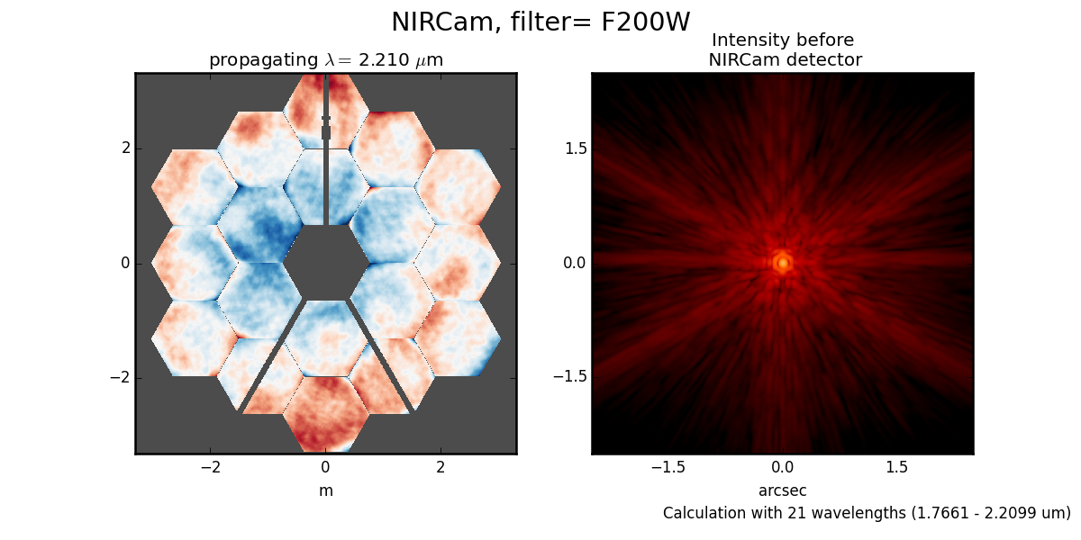
Instantiate a model of NIRCam, set attributes to configure a particular observing mode, then call calc_psf():

>>> import webbpsf
>>> nc = webbpsf.NIRCam()
>>> nc.filter =  'F200W'
>>> psf = nc.calc_psf(oversample=4)     # returns an astropy.io.fits.HDUlist containing PSF and header
>>> plt.imshow(psf[0].data)             # display it on screen yourself, or
>>> webbpsf.display_psf(psf)            # use this convenient function to make a nice log plot with labeled axes
>>>
>>> nc.calc_psf("myPSF.fits")         # you can also write the output directly to disk if you prefer.

For interactive use, you can have the PSF displayed as it is computed:

>>> nc.calc_psf(display=True)                          # will make nice plots with matplotlib.

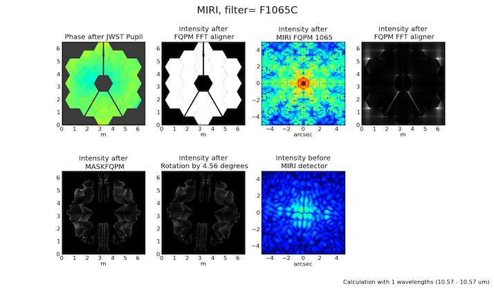
More complicated instrumental configurations are available by setting the instrument’s attributes. For instance, one can create an instance of MIRI and configure it for coronagraphic observations, thus:

>>> miri = webbpsf.MIRI()
>>> miri.filter = 'F1065C'
>>> miri.image_mask = 'FQPM1065'
>>> miri.pupil_mask = 'MASKFQPM'
>>> miri.calc_psf('outfile.fits')

Input Source Spectra

WebbPSF attempts to calculate realistic weighted broadband PSFs taking into account both the source spectrum and the instrumental spectral response.

The default source spectrum is, if synphot is installed, a G2V star spectrum from Castelli & Kurucz 2004. Without synphot, the default is a simple flat spectrum such that the same number of photons are detected at each wavelength.

You may choose a different illuminating source spectrum by specifying a source parameter in the call to calc_psf(). The following are valid sources:

1. A synphot.SourceSpectrum object. This is the best option, providing maximum ease and accuracy, but requires the user to have synphot installed. In this case, the SourceSpectrum object is combined with a synphot.SpectralElement for the selected instrument and filter to derive the effective stimulus in detected photoelectrons versus wavelength. This is binned to the number of wavelengths set by the nlambda parameter.

2. A dictionary with elements source["wavelengths"] and source["weights"] giving the wavelengths in meters and the relative weights for each. These should be numpy arrays or lists. In this case, the wavelengths and weights are used exactly as provided, without applying the instrumental filter profile.

   >>> src = {'wavelengths': [2.0e-6, 2.1e-6, 2.2e-6], 'weights': [0.3, 0.5, 0.2]}
   >>> nc.calc_psf(source=src, outfile='psf_for_src.fits')
   

3. A tuple or list containing the numpy arrays (wavelength, weights) instead.

As a convenience, webbpsf includes a function to retrieve an appropriate synphot.SourceSpectrum object for a given stellar spectral type from the PHOENIX or Castelli & Kurucz model libraries.

>>> src = webbpsf.specFromSpectralType('G0V', catalog='phoenix')
>>> psf = miri.calc_psf(source=src)

Making Monochromatic PSFs

To calculate a monochromatic PSF, just use the monochromatic parameter. Wavelengths are always specified in meters.

>>> psf = miri.calc_psf(monochromatic=9.876e-6)

Adjusting source position, centering, and output format

A number of non-instrument-specific calculation options can be adjusted through the options dictionary attribute on each instrument instance. (For a complete listing of options available, consult JWInstrument.options.)

Input Source position offsets

The PSF may be shifted off-center by adjusting the offset of the stellar source. This is done in polar coordinates:

>>> instrument.options['source_offset_r'] = 0.3         # offset in arcseconds
>>> instrument.options['source_offset_theta'] = 45.     # degrees counterclockwise from instrumental +Y in the science frame

For convenience offsets can also be given in cartesian coordinates:

>>> instrument.options['source_offset_x'] = 4        # offset is in arsec
>>> instrument.options['source_offset_y'] = -3     # offset is in arsec

The option source_offset defines “the location of the point source within the simulated subarray”. It doesn’t affect the WFE, but it does affect the position offset of the source relative to any focal plane elements such as a coronagraph mask or spectrograph slit. For coronagraphic modes, the coronagraph occulter is always assumed to be at the center of the output array. Therefore, these options let you offset the source away from the coronagraph.

Note that instead of offsetting the source we could offset the coronagraph mask in the opposite direction. This can be done with the coron_shift_x and coron_shift_y options. These options will offset a coronagraphic mask in order to produce PSFs centered in the output image, rather than offsetting the PSF. Both options, coron_shift and source_offset give consistent results. Using the same source_offset values above, we can use offset a coronagraphic mask:

>>> instrument.options['coron_shift_x'] = -4        # offset is in arsec, note opposite sign convention
>>> instrument.options['coron_shift_y'] = +3     # offset is in arsec, note opposite sign convention

If these options are set, the offset is applied relative to the central coordinates as defined by the output array size and parity (described just below).

Simulating telescope jitter

Space-based observatories don’t have to contend with the seeing limit, but imprecisions in telescope pointing can have the effect of smearing out the PSF. To simulate this with WebbPSF, the option names are jitter and jitter_sigma.

>>> instrument.options['jitter'] = 'gaussian'   # jitter model name or None
>>> instrument.options['jitter_sigma'] = 0.009  # in arcsec per axis, default 0.007

Array sizes, star positions, and centering

Output array sizes may be specified either in units of arcseconds or pixels. For instance,

>>> mynircam = webbpsf.NIRCam()
>>> mynircam.filter = 'F250M'
>>> result = mynircam.calc_psf(fov_arcsec=7, oversample=2)
>>> result2= mynircam.calc_psf(fov_pixels=512, oversample=2)

In the latter example, you will in fact get an array which is 1024 pixels on a side: 512 physical detector pixels, times an oversampling of 2.

By default, the PSF will be centered at the exact center of the output array. This means that if the PSF is computed on an array with an odd number of pixels, the PSF will be centered exactly on the central pixel. If the PSF is computed on an array with even size, it will be centered on the “crosshairs” at the intersection of the central four pixels. If one of these is particularly desirable to you, set the parity option appropriately:

>>>  instrument.options['parity'] = 'even'
>>>  instrument.options['parity'] = 'odd'

Setting one of these options will ensure that a field of view specified in arcseconds is properly rounded to either odd or even when converted from arcsec to pixels. Alternatively, you may also just set the desired number of pixels explicitly in the call to calc_psf():

>>>  instrument.calc_psf(fov_pixels=512)

Note

Please note that these parity options apply to the number of detector pixels in your simulation. If you request oversampling, then the number of pixels in the output file for an oversampled array will be fov_npixels times oversampling. Hence, if you request an odd parity with an even oversampling of, say, 4, then you would get an array with a total number of data pixels that is even, but that correctly represents the PSF located at the center of an odd number of detector pixels.

Output format options for sampling

As just explained, WebbPSF can easily calculate PSFs on a finer grid than the detector’s native pixel scale. You can select whether the output data should include this oversampled image, a copy that has instead been rebinned down to match the detector scale, or optionally both. This is done using the options['output_mode'] parameter.

>>> nircam.options['output_mode'] = 'oversampled'
>>> psf = nircam.calc_psf()       # the 'psf' variable will be an oversampled PSF, formatted as a FITS HDUlist
>>>
>>> nircam.options['output_mode'] = 'detector sampled'
>>> psf2 = nircam.calc_psf()      # now 'psf2' will contain the result as resampled onto the detector scale.
>>>
>>> nircam.options['output_mode'] = 'both'
>>> psf3 = nircam.calc_psf()      # 'psf3' will have the oversampled image as primary HDU, and
>>>                              # the detector-sampled image as the first image extension HDU.

Warning

The default behavior is both. Note that at some point in the future, this default is likely to change to detector sampling. To future-proof your code, set options['output_mode'] explicitly.

Pixel scales, sampling, and oversampling

The derived instrument classes all know their own instrumental pixel scales. You can change the output pixel scale in a variety of ways, as follows. See the JWInstrument.calc_psf documentation for more details.

1. Set the oversample parameter to calc_psf(). This will produce a PSF with a pixel grid this many times more finely sampled. oversample=1 is the native detector scale, oversample=2 means divide each pixel into 2x2 finer pixels, and so forth.

   >>> hdulist = instrument.calc_psf(oversample=2)    # hdulist will contain a primary HDU with the
   >>>                                                # oversampled data
   

2. For coronagraphic calculations, it is possible to set different oversampling factors at different parts of the calculation. See the fft_oversample and detector_oversample parameters. This is of no use for regular imaging calculations (in which case oversample is a synonym for detector_oversample). Specifically, the fft_oversample keyword is used for Fourier transformation to and from the intermediate optical plane where the occulter (coronagraph spot) is located, while detector_oversample is used for propagation to the final detector. Note that the behavior of these keywords changes for coronagraphic modeling using the Semi-Analytic Coronagraphic propagation algorithm (not fully documented yet - contact Marshall Perrin if curious).

   >>> miri.calc_psf(fft_oversample=8, detector_oversample=2)  # model the occulter with very fine pixels, then save the
   >>>                                                          # data on a coarser (but still oversampled) scale
   

3. Or, if you need even more flexibility, just change the instrument.pixelscale attribute to be whatever arbitrary scale you require.

   >>> instrument.pixelscale = 0.0314159
   

Note that the calculations performed by WebbPSF are somewhat memory intensive, particularly for coronagraphic observations. All arrays used internally are double-precision complex floats (16 bytes per value), and many arrays of size (npixels * oversampling)^2 are needed (particularly if display options are turned on, since the matplotlib graphics library makes its own copy of all arrays displayed).

Your average laptop with a couple GB of RAM will do perfectly well for most computations so long as you’re not too ambitious with setting array size and oversampling. If you’re interested in very high fidelity simulations of large fields (e.g. 1024x1024 pixels oversampled 8x) then we recommend a large multicore desktop with >16 GB RAM.

PSF normalization

By default, PSFs are normalized to total intensity = 1.0 at the entrance pupil (i.e. at the JWST OTE primary). A PSF calculated for an infinite aperture would thus have integrated intensity =1.0. A PSF calculated on any smaller finite subarray will have some finite encircled energy less than one. For instance, at 2 microns a 10 arcsecond size FOV will enclose about 99% of the energy of the PSF. Note that if there are any additional obscurations in the optical system (such as coronagraph masks, spectrograph slits, etc), then the fraction of light that reaches the final focal plane will typically be significantly less than 1, even if calculated on an arbitrarily large aperture. For instance the NIRISS NRM mask has a throughput of about 15%, so a PSF calculated in this mode with the default normalization will have integrated total intensity approximately 0.15 over a large FOV.

If a different normalization is desired, there are a few options that can be set in calls to calc_psf:

>>>  psf = nc.calc_psf(normalize='last')

The above will normalize a PSF after the calculation, so the output (i.e. the PSF on whatever finite subarray) has total integrated intensity = 1.0.

>>>  psf = nc.calc_psf(normalize='exit_pupil')

The above will normalize a PSF at the exit pupil (i.e. last pupil plane in the optical model). This normalization takes out the effect of any pupil obscurations such as coronagraph masks, spectrograph slits or pupil masks, the NIRISS NRM mask, and so forth. However it still leaves in the effect of any finite FOV. In other words, PSFs calculated in this mode will have integrated total intensity = 1.0 over an infinitely large FOV, even after the effects of any obscurations.

Note

An aside on throughputs and normalization: Note that by design WebbPSF does not track or model the absolute throughput of any instrument. Consult the JWST Exposure Time Calculator and associated reference material if you are interested in absolute throughputs. Instead WebbPSF simply allows normalization of output PSFs’ total intensity to 1 at either the entrance pupil, exit pupil, or final focal plane. When used to generate monochromatic PSFs for use in the JWST ETC, the entrance pupil normalization option is selected. Therefore WebbPSF first applies the normalization to unit flux at the primary mirror, propagates it through the optical system ignoring any reflective or transmissive losses from mirrors or filters (since the ETC throughput curves take care of those), and calculates only the diffractive losses from slits and stops. Any loss of light from optical stops (Lyot stops, spectrograph slits or coronagraph masks, the NIRISS NRM mask, etc.) will thus be included in the WebbPSF calculation. Everything else (such as reflective or transmissive losses, detector quantum efficiencies, etc., plus scaling for the specified target spectrum and brightness) is the ETC’s job. This division of labor has been coordinated with the ETC team and ensures each factor that affects throughput is handled by one or the other system but is not double counted in both.

To support realistic calculation of broadband PSFs however, WebbPSF does include normalized copies of the relative spectral response functions for every filter in each instrument. These are included in the WebbPSF data distribution, and are derived behind the scenes from the same reference database as is used for the ETC. These relative spectral response functions are used to make a proper weighted sum of the individual monochromatic PSFs in a broadband calculation: weighted relative to the broadband total flux of one another, but still with no implied absolute normalization.

Controlling output log text

WebbPSF can output a log of calculation steps while it runs, which can be displayed to the screen and optionally saved to a file. This is useful for verifying or debugging calculations. To turn on log display, just run

>>> webbpsf.setup_logging(filename='webbpsf.log')

The setup_logging function allows selection of the level of log detail following the standard Python logging system (DEBUG, INFO, WARN, ERROR). To disable all printout of log messages, except for errors, set

>>> webbpsf.setup_logging(level='ERROR')

WebbPSF remembers your chosen logging settings between invocations, so if you close and then restart python it will automatically continue logging at the same level of detail as before. See webbpsf.setup_logging() for more details.

Advanced Usage: Output file format, OPDs, and more

This section serves as a catch-all for some more esoteric customizations and applications. See also the More Examples page.

Writing out only downsampled images

Perhaps you may want to calculate the PSF using oversampling, but to save disk space you only want to write out the PSF downsampled to detector resolution.

>>> result =  inst.calc_psf(args, ...)
>>> result['DET_SAMP'].writeto(outputfilename)

Or if you really care about writing it as a primary HDU rather than an extension, replace the 2nd line with

>>> pyfits.PrimaryHDU(data=result['DET_SAMP'].data, header=result['DET_SAMP'].header).writeto(outputfilename)

Writing out intermediate images

Your calculation may involve intermediate pupil and image planes (in fact, it most likely does). WebbPSF / POPPY allow you to inspect the intermediate pupil and image planes visually with the display keyword argument to calc_psf(). Sometimes, however, you may want to save these arrays to FITS files for analysis. This is done with the save_intermediates keyword argument to calc_psf().

The intermediate wavefront planes will be written out to FITS files in the current directory, named in the format wavefront_plane_%03d.fits. You can additionally specify what representation of the wavefront you want saved with the save_intermediates_what argument to calc_psf(). This can be all, parts, amplitude, phase or complex, as defined as in poppy.Wavefront.asFITS(). The default is to write all (intensity, amplitude, and phase as three 2D slices of a data cube).

If you pass return_intermediates=True as well, the return value of calc_psf is then psf, intermediate_wavefronts_list rather than the usual psf.

Warning

The save_intermediates keyword argument does not work when using parallelized computation, and WebbPSF will fail with an exception if you attempt to pass save_intermediates=True when running in parallel. The return_intermediates option has this same restriction.

Providing your own OPDs or pupils from some other source

It is straight forward to configure an Instrument object to use a pupil OPD file of your own devising, by setting the pupilopd attribute of the Instrument object:

>>> niriss = webbpsf.NIRISS()
>>> niriss.pupilopd = "/path/to/your/OPD_file.fits"

If you have a pupil that is an array in memory but not saved on disk, you can pass it in as a fits.HDUList object :

>>> myOPD = some_function_that_returns_properly_formatted_HDUList(various, function, args...)
>>> niriss.pupilopd = myOPD

Likewise, you can set the pupil transmission file in a similar manner by setting the pupil attribute:

>>> niriss.pupil = "/path/to/your/OPD_file.fits"

Please see the documentation for poppy.FITSOpticalElement for information on the required formatting of the FITS file. In particular, you will need to set the PUPLSCAL keyword, and OPD values must be given in units of meters.

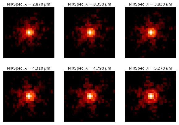
Calculating Data Cubes

Sometimes it is convenient to calculate many PSFs at different wavelengths with the same instrument config. You can do this just by iterating over calls to calc_psf, but there’s also a function to automate this: calc_datacube. For example, here’s something loosely like the NIRSpec IFU in F290LP:

# Set up a NIRSpec instance
nrs = webbpsf.NIRSpec()
nrs.image_mask = None # No MSA for IFU mode
nl = np.linspace(2.87e-6, 5.27e-6, 6)

# Calculate PSF datacube
cube = nrs.calc_datacube(wavelengths=nl, fov_pixels=27, oversample=4)

# Display the contents of the data cube
fig, axes = plt.subplots(nrows=2, ncols=3, figsize=(10,7))
for iy in range(2):
    for ix in range(3):
        ax=axes[iy,ix]
        i = iy*3+ix
        wl = cube[0].header['WAVELN{:02d}'.format(i)]

        # Note that when displaying datacubes, you have to set the "cube_slice" parameter
        webbpsf.display_psf(cube, ax=ax, cube_slice=i,
                            title="NIRSpec, $\lambda$ = {:.3f} $\mu$m".format(wl*1e6),
                            vmax=.2, vmin=1e-4, ext=1, colorbar=False)
        ax.xaxis.set_visible(False)
        ax.yaxis.set_visible(False)

Subclassing a JWInstrument to add additional functionality

Perhaps you want to modify the OPD used for a given instrument, for instance to add a defocus. You can do this by subclassing one of the existing instrument classes to override the JWInstrument._addAdditionalOptics() function. An OpticalSystem is basically a list so it’s straightforward to just add another optic there. In this example it’s a lens for defocus but you could just as easily add another FITSOpticalElement instead to read in a disk file.

Note, we do this as an example here to show how to modify an instrument class by subclassing it, which can let you add arbitrary new functionality. There’s an easier way to add defocus specifically; see below.

>>> class FGS_with_defocus(webbpsf.FGS):
>>>     def __init__(self, *args, **kwargs):
>>>         webbpsf.FGS.__init__(self, *args, **kwargs)
>>>         # modify the following as needed to get your desired defocus
>>>         self.defocus_waves = 0
>>>         self.defocus_lambda = 4e-6
>>>     def _addAdditionalOptics(self, optsys, *args, **kwargs):
>>>         optsys = webbpsf.FGS._addAdditionalOptics(self, optsys, *args, **kwargs)
>>>         lens = poppy.ThinLens(
>>>             name='FGS Defocus',
>>>             nwaves=self.defocus_waves,
>>>             reference_wavelength=self.defocus_lambda
>>>         )
>>>         lens.planetype = poppy.PUPIL  # tell propagation algorithm which this is
>>>         optsys.planes.insert(1, lens)
>>>         return optsys
>>>
>>> fgs2 = FGS_with_defocus()
>>> # apply 4 waves of defocus at the wavelength
>>> # defined by FGS_with_defocus.defocus_lambda
>>> fgs2.defocus_waves = 4
>>> psf = fgs2.calc_psf()
>>> webbpsf.display_psf(psf)

Defocusing an instrument

The instrument options dictionary also lets you specify an optional defocus amount. You can specify both the wavelength at which it should be applied, and the number of waves of defocus (at that wavelength, specified as waves peak-to-valley over the circumscribing circular pupil of JWST).

>>> nircam.options['defocus_waves'] = 3.2
>>> nircam.options['defocus_wavelength'] = 2.0e-6