JWST Using Wavefronts Measured On Orbit
WebbPSF now includes code for using the results of in-flight wavefront sensing measurements, by retrieving Optical Path Difference (OPD) files which include the sensing results for the positions of the mirrors at different times. These are produced by the JWST Wavefront Sensing Subsystem (WSS), using focus diverse phase retrieval on NIRCam weak lens data taken roughly every two days in flight. The output OPDs from that are saved in MAST and can be automatically retrieved and used in WebbPSF.
Begin by instantiating an instrument instance in the usual manner. In this case, let’s set up a NIRCam instance for one of the detectors in module B.
[2]:
nrc = webbpsf.NIRCam()
nrc.filter='F200W'

nrc.detector = 'NRCB2'
nrc.detector_position = (1024,1024)
Finding the measured wavefront near a given date
To load an OPD corresponding to observations on some particular date, use the method load_wss_opd_by_date. This takes as its first argument a date time specified in ISO format, like “YYYY-MM-DDTHH:MM:SS”.
Let’s also set plot=True so this makes a plot which shows what’s going on.
[3]:
nrc.load_wss_opd_by_date('2022-07-01T00:00:00',plot=True)
MAST OPD query around UTC: 2022-07-01T00:00:00.000
                        MJD: 59761.0

OPD immediately preceding the given datetime:
        URI:     mast:JWST/product/R2022063002-NRCA3_FP1-2.fits
        Date (MJD):      59759.6628
        Delta time:      -1.3372 days

OPD immediately following the given datetime:
        URI:     mast:JWST/product/R2022070403-NRCA3_FP1-0.fits
        Date (MJD):      59761.5484
        Delta time:      0.5484 days
User requested choosing OPD time closest in time to 2022-07-01T00:00:00.000, which is R2022070403-NRCA3_FP1-0.fits, delta time 0.548 days
Importing and format-converting OPD from /Users/mperrin/software/webbpsf-data/MAST_JWST_WSS_OPDs/R2022070403-NRCA3_FP1-0.fits
Backing out SI WFE and OTE field dependence at the WF sensing field point
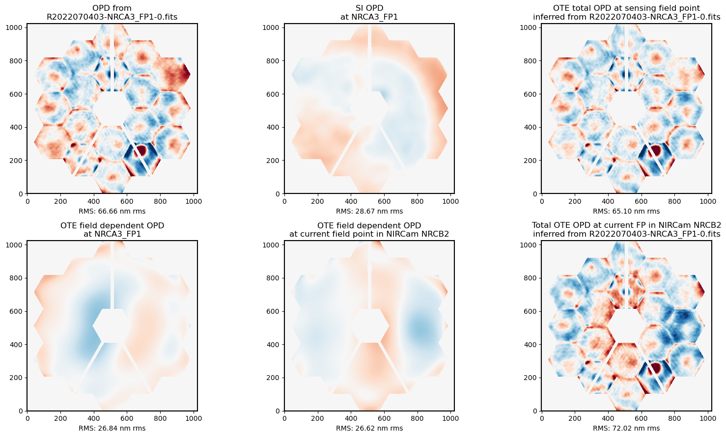
Given the input date, the function queries to find the closest-in-time wavefront sensing result. In this case it is a measurement about 0.5 days after the specified time. (You can set keyword choice='before' or choice='after' if you have some reason to specify which in particular). That OPD file will be automatically retrievd from MAST; downloads are cached inside your $WEBBPSF_DATA_PATH directory for reuse in multiple calculations.
Let’s look at each plot in turn.
Upper Left: This is the measured OPD as sensed in NIRCam at “field point 1” which is in the upper left corner of NRCA3, relatively close to the center of the NIRCam module. This observatory total OPD measurement includes both the telescope and NIRCam contributions to the WFE.
Upper Middle: This is the wavefront map for the NIRCam portion of the WFE at that field point. This is known from ground calibration test data, not measured in flight.
Upper Right: That NIRCam WFE contribution is subtracted from the total observatory WFE to yield this estimate of the OTE-only portion of the WFE.
Lower Left and Middle: These are models for the field dependence of the OTE OPD between the sensing field point in NRCA3 and the requested field ooint, in this case in NRCB2. This field dependence arises mostly from the figure of the tertiary mirror. These are used to transform the estimated OTE OPD from one field position to another.
Lower Right: This is the resulting estimate for the OTE OPD at the requested field point, in this case in NRCB2.
All those calculations happen automatically as part of the load_wss_opd_by_date (inside the load_wss_opd function which it calls in turn).
After that it’s just a matter of calculating PSFs as usual:
[4]:
psf = nrc.calc_psf(fov_pixels=101)
[5]:
plt.figure(figsize=(16,9))
webbpsf.display_psf(psf, ext=1)
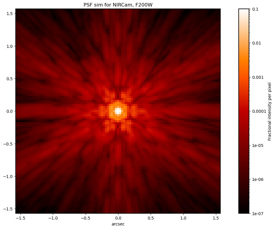
Thus, the above PSF is calculated using the actual as-measured-at-L2 state of the telescope WFE near the requested date, in this case 2022 July 1.
Loading a particular OPD file
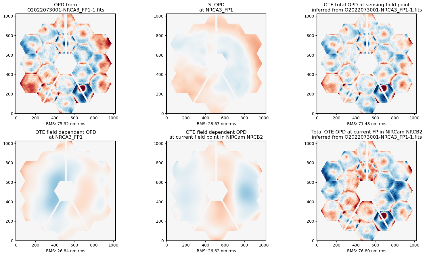
If you already know the filename of a particular desired OPD file, you can simply retrieve it by name using the load_wss_opd function. Once again, this file will be automatically retrieved from MAST if necessary.
[6]:
nrc.load_wss_opd("O2022073001-NRCA3_FP1-1.fits", plot=True)
Found OPD file previously downloaded: O2022073001-NRCA3_FP1-1.fits
Importing and format-converting OPD from /Users/mperrin/software/webbpsf-data/MAST_JWST_WSS_OPDs/O2022073001-NRCA3_FP1-1.fits
Backing out SI WFE and OTE field dependence at the WF sensing field point
Trending Wavefront Changes over Time
To help observers understand how the mirror alignments change over time, and when such changes might affect PSFs in science data, WebbPSF also includes some functions for generating trending plots showing wavefronts over time.
These functions work by downloading sets of several OPDs from MAST, and performing calculations such as inferring the changes between one measurement and the next.
Wavefront Trending throughout a given month
A wavefront trending plot can be produced that shows wavefront changes during some particular month of interest:
[7]:
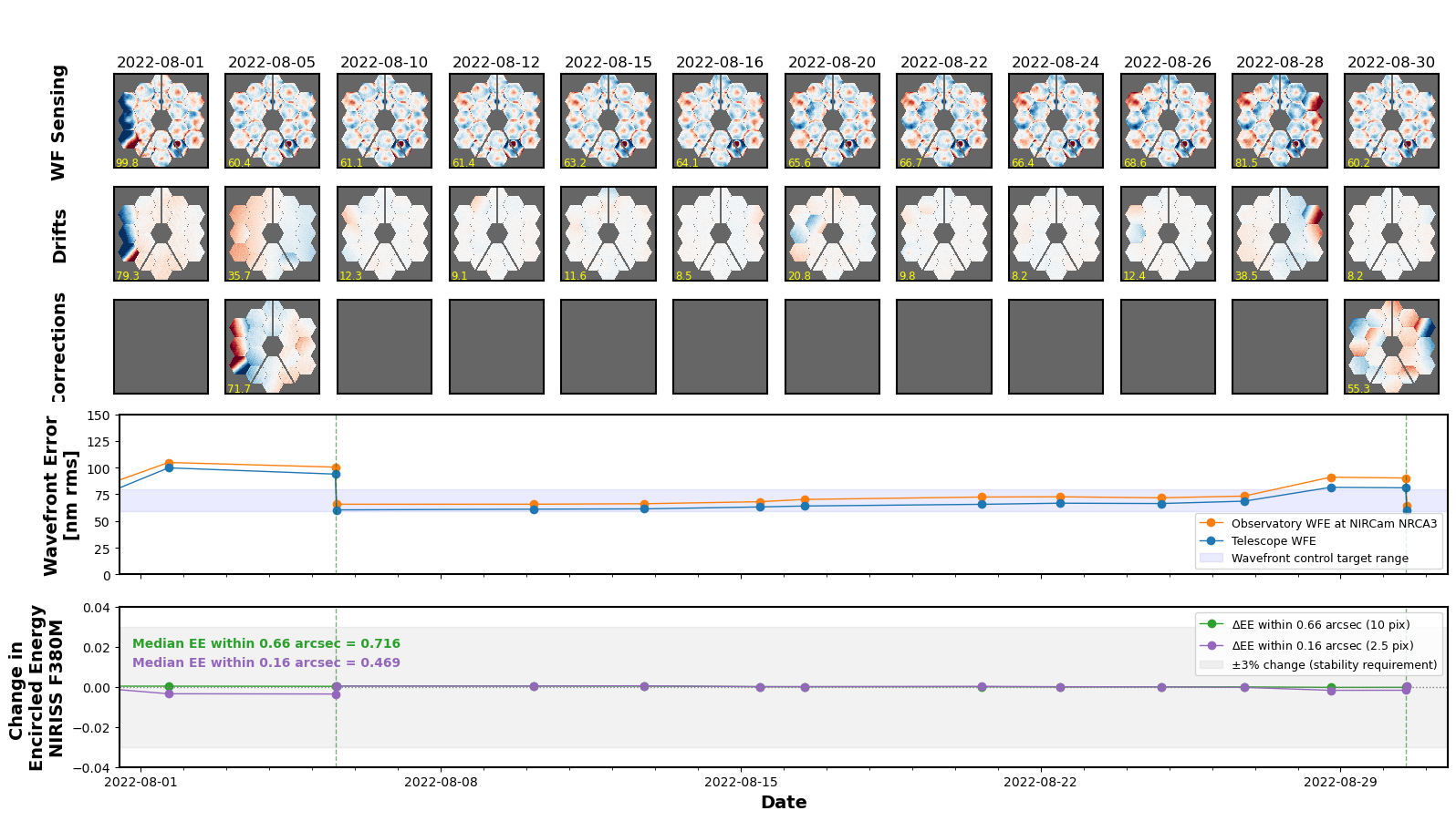
trend_table = webbpsf.trending.monthly_trending_plot(2022, 8, verbose=False)
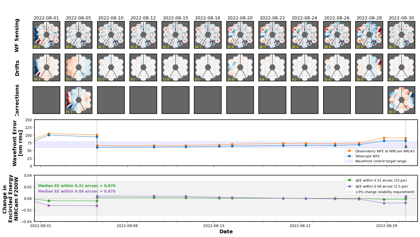
The above figure shows:
Each wavefront sensing measurement throughout the specified month (first row)
The drift in wavefront between each two successive measurements (i.e. the changes arising in the telescope itself, without any ground commanding. Second row)
The mirror corrections applied (i.e. the result of mirror move commands sent from the ground. Third row)
Plots of the wavefront RMS value over time, for both the OTE wavefront only (i.e. the waveront quality from the telescope delivered to the NIRCam sensing field point) and the total observatory wavefront (i.e. the sum of telescope and instrument contributions to the wavefront).
Computed values for the encircled energy within radii of 2.5 pixels and 10 pixels, and their variation over time.
In the above plot for 2022 July, we can see that the wavefront was generally stable (very little change from one meaurement to the next, but a few individual mirror tilt events can be seen for instance in the July 4 and July 6 sensing). A wavefront correction was applied on July 8. Then the July 12 wavefront sensing revealed a larger wing tilt event affecting the several segments on the left (-V2) wing. This was corrected in the July 15 wavefront sensing and control observation, and after that the telescope remained stable throughout the rest of that month’s wavefront sensing.
The monthly_trending_plot function automatically saves the plot as a PDF to the current working directory, with filenames like “wf_trending_2022-08.pdf'”
The function also returns a table with information summarizing the available WFS measurements, WFE levels, and computed PSF encircle energies. This can be used to help understand how much the photometry in your observation is affected by PSF changes at a given time.
[8]:
trend_table
[8]:
| Date | Filename | WFS Type | RMS WFE (OTE+SI) | RMS WFE (OTE only) | EE(2.5 pix) | EE(10pix) |
|---|---|---|---|---|---|---|
| nm | nm | |||||
| str23 | str29 | str16 | float64 | float64 | float64 | float64 |
| 2022-07-30T14:16:12.800 | O2022073001-NRCA3_FP1-1.fits | Sensing | 75.3218690264774 | 66.09542450712576 | 0.6696332020294565 | 0.8767156339082203 |
| 2022-08-01T15:29:51.000 | R2022080204-NRCA3_FP1-0.fits | Sensing | 104.78028353286832 | 99.77286798005535 | 0.6569210392362466 | 0.871685491787062 |
| 2022-08-05T12:55:58.900 | R2022080601-NRCA3_FP1-0.fits | Sensing | 100.43731215562515 | 93.88799015744388 | 0.6565941724030266 | 0.8715130503124521 |
| 2022-08-05T13:38:34.300 | R2022080601-NRCA3_FP1-1.fits | Post Mirror Move | 65.70009131907837 | 60.41040935551668 | 0.6733419027570456 | 0.8771249633140422 |
| 2022-08-10T04:06:35.800 | R2022081102-NRCA3_FP1-1.fits | Sensing | 65.7455043858421 | 61.08067782976896 | 0.6732164429302696 | 0.8770853234542049 |
| 2022-08-12T17:58:37.000 | O2022081401-NRCA3_FP1-1.fits | Sensing | 66.18345915687821 | 61.35862651863206 | 0.672807234955758 | 0.8769571339901217 |
| 2022-08-15T10:41:30.900 | O2022081601-NRCA3_FP1-1.fits | Sensing | 68.05351480352284 | 63.17040406499793 | 0.671085164794359 | 0.8761902354255183 |
| 2022-08-16T11:38:59.500 | O2022081602-NRCA3_FP1-1.fits | Sensing | 70.1897000850969 | 64.05438013560472 | 0.6708090590535625 | 0.87618409429269 |
| 2022-08-20T14:48:34.300 | R2022082003-NRCA3_FP1-1.fits | Sensing | 72.44368124558385 | 65.63411445402757 | 0.6695446822188404 | 0.8760920643391353 |
| 2022-08-22T10:53:59.300 | R2022082202-NRCA3_FP1-1.fits | Sensing | 72.68510003044359 | 66.67806803793583 | 0.6689157923113629 | 0.8757979843558308 |
| 2022-08-24T19:21:06.100 | R2022090101-NRCA3_FP1-2.fits | Sensing | 71.72083328054846 | 66.37091153605623 | 0.6684202360216875 | 0.8759543259835378 |
| 2022-08-26T17:58:13.600 | R2022082702-NRCA3_FP1-1.fits | Sensing | 73.33806334948196 | 68.55067517101686 | 0.6680685210194995 | 0.8758259956765841 |
| 2022-08-28T18:26:59.700 | R2022082903-NRCA3_FP1-0.fits | Sensing | 91.00956623974646 | 81.52170528385567 | 0.661149397592053 | 0.8742555503448957 |
| 2022-08-30T12:22:42.100 | R2022090102-NRCA3_FP1-1.fits | Sensing | 90.24298317520685 | 81.08651132830643 | 0.6614514775697193 | 0.8744257093115919 |
| 2022-08-30T13:11:54.700 | R2022083109-NRCA3_FP1-1.fits | Post Mirror Move | 64.66059678377493 | 60.1907903724738 | 0.672899177019872 | 0.8778265977632995 |
By default, the trending table performs computations of the encircled energy for NIRCam F200W, but you can specify a different instrument and filter if so desired.
[9]:
webbpsf.trending.monthly_trending_plot(2022, 8, verbose=False, instrument='NIRISS', filter='F380M');
Wavefront time series and histogram plots
Other functions can provide views of wavefront changes over even longer timescales. We can retrieve a table of all available OPDs and plot the measurements over time:
[2]:
opdtable = webbpsf.mast_wss.retrieve_mast_opd_table()
opdtable = webbpsf.mast_wss.deduplicate_opd_table(opdtable)
webbpsf.mast_wss.download_all_opds(opdtable)
[3]:
webbpsf.trending.wavefront_time_series_plot(opdtable)
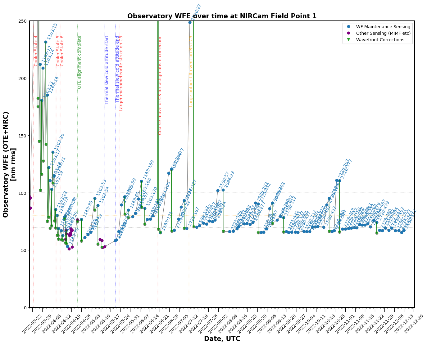
The above shows wavefront drifts and corrections from around the middle of OTE commissioning to the early part of Cycle 1. Rapid drifts and corrections in early March are from the MIRI cryocooler gradually cooling the observatory, until reaching thermal stability in mid April.
Occasional increases in wavefront error from mirror tilts and corrections can be seen in subsequent months. There was an especially large tilt event on July 12, which was corrected on July 15.
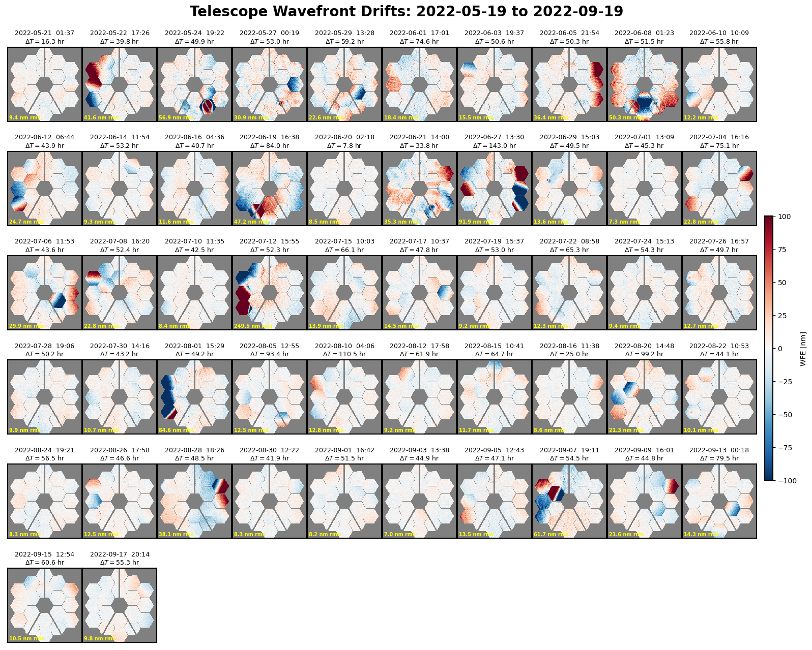
We can also plot all measured wavefront drifts over specified time periods.
[4]:
start_time =  astropy.time.Time('2022-05-19T00:00:00')
end_time = astropy.time.Time('2022-09-19T00:00:00')

webbpsf.trending.wavefront_drift_plots(opdtable, start_time=start_time, end_time=end_time, n_per_row=10)
Lastly, we can plot histograms of wavefront error levels over time.
[5]:
start_time =  astropy.time.Time('2022-07-16')
webbpsf.trending.wfe_histogram_plot(opdtable, thresh=80, mark_corrections='arrows')
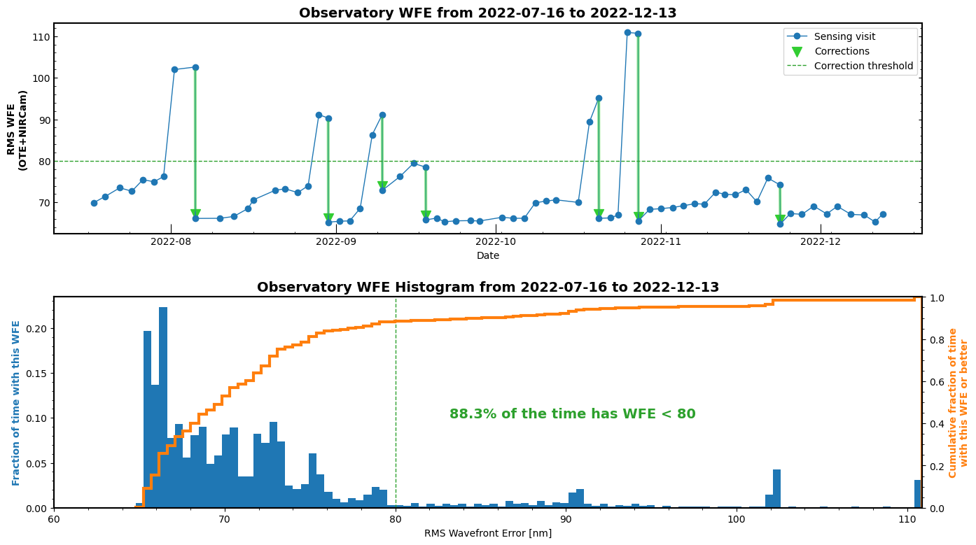
The above plot shows the wavefront error evolution over the first part of Cycle 1, starting after the ERO release on July 12 and continuing up to present (as of 2022 Dec 13, during the “First Science with JWST” conference). You can see the occasional larger tilt events which are subsequently detected and corrected. It appears possible that the frequency of the larger events may be decreasing over time.
[ ]:
Viewing wavefront observation data and deltas
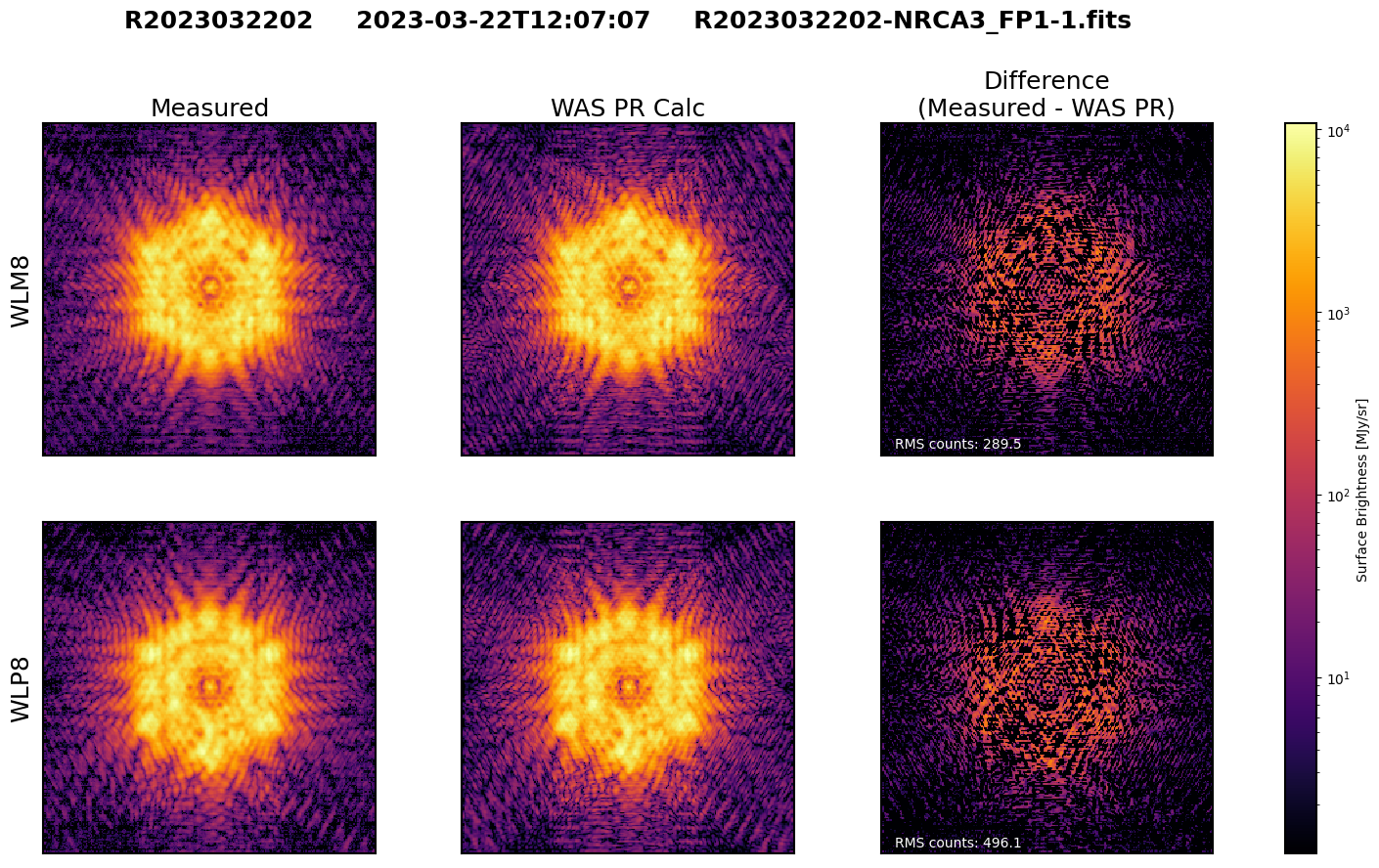
In addition to the derived wavefront maps, the OPD data files in MAST contain FITS extensions with the image data from the wavefront sensing measurements, with cutouts of the weak lens sensing data. (The full images are also separately available from MAST too). Although most users will not need to refer to these, WebbPSF includes display tools for viewing them, for instance to help cross-check the quality of a particular wavefront retrieval.
The function plot_phase_retrieval_crosscheck shows the measured weak lens data (left column), and the models of these produced by the Wavefront Analysis Software during the phase retrieval analyses (middle column).
[3]:
most_recent_wfs_file = opdtable[-1]['fileName']

webbpsf.trending.plot_phase_retrieval_crosscheck(most_recent_wfs_file);
<Figure size 640x480 with 0 Axes>
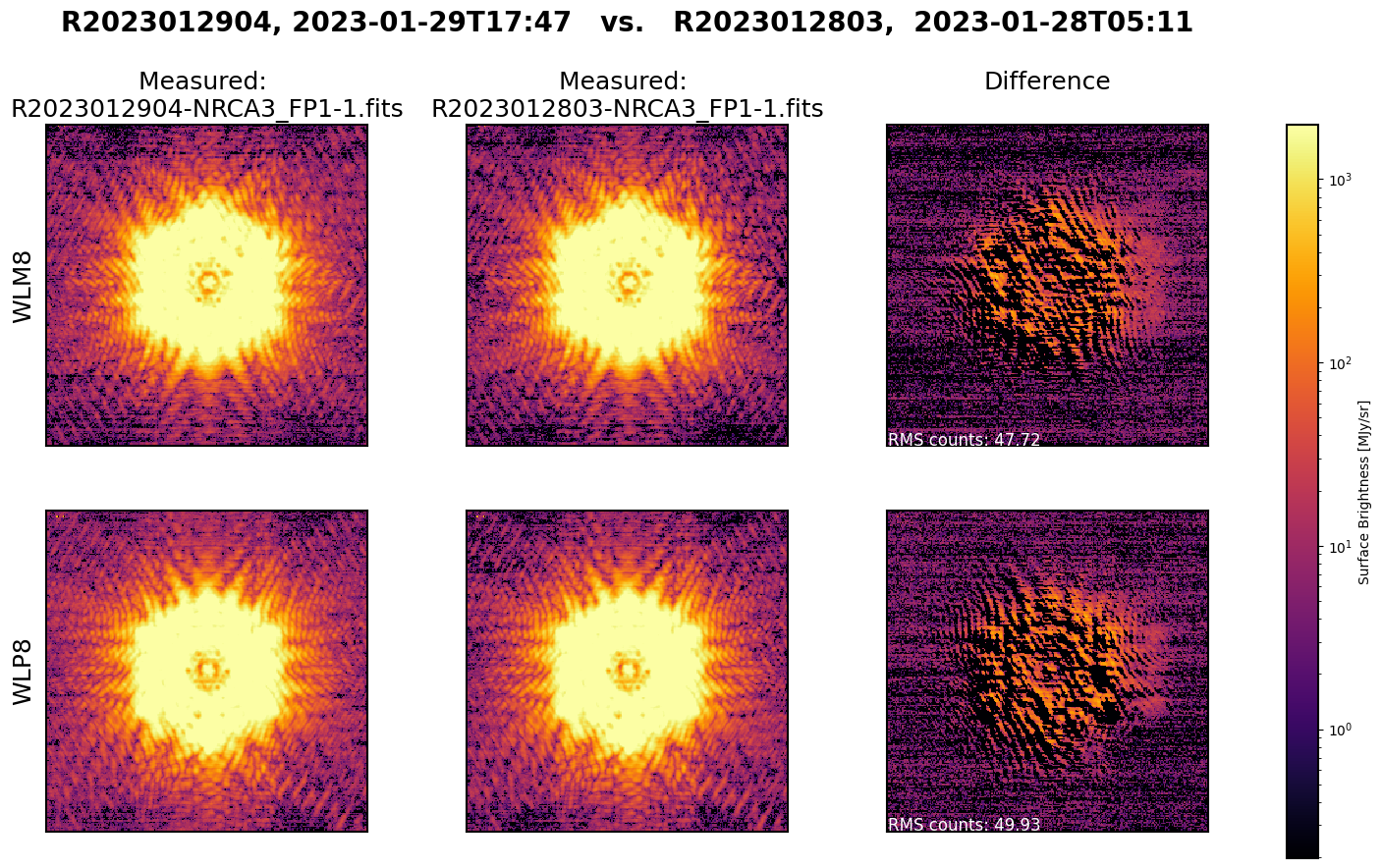
The function plot_wfs_obs_delta plots the difference of two (probably successive) WFS observations. This can be a useful way to quickly visualize what changed from one observation to another, including the presence of potential spoilers such as binary companions.
Here’s an example of that from WF sensing in January 2023. The presence of a binary companion shows up clearly in the difference image.
[4]:
webbpsf.trending.plot_wfs_obs_delta('R2023012904-NRCA3_FP1-1.fits', 'R2023012803-NRCA3_FP1-1.fits',
                                    vmax_fraction=0.2);
<Figure size 640x480 with 0 Axes>
[ ]: